Because if two models are better than one, then surely a whole heap of models are better still.

Jupyter notebooks used for this post can be found here.
Of encapsulation and densification
When I started on my project to build a new footy-tipping model, one of my principle ideas was to achieve greater accuracy by building a modular ensemble model, one whose individual pieces functioned as independent models, each with its own data source, whose predictions would be combined only at the very end of the data pipeline. I was inspired to try out this structure from studying the principles and best practices of object-oriented programming. (For those who are interested, Sandi Metz’s *Practical Object-Oriented Design* is an excellent introduction.) I figured that reducing the interdependence of different sections of a codebase for greater flexibility and openness to change is as useful to a machine learning project as it is to a web application. Another influence was the limitations of the data itself: I have match data going back to 1897, (useful) player data going back to 1965, and betting data going back to 2010. Joining all of these together results in a sparse data table, especially since there’s a negative correlation between a data column’s length and its importance to a model’s predictions. The betting odds are some of the strongest predictors of which team will win, because they include the collected wisdom of experts and fans into a few numbers, but I only have these valuable figures for 12.2% of my data rows. My thinking was that reducing the sparsity of my data by splitting it up by type (betting, player, match) would reduce the amount of noise (i.e. zeros) and enhance my model’s ability to learn the values that were present. In pursuit of this idea, I’ve created a model trained on betting data only, one trained on player data only, one trained on match data only, and now I’m ready to bring them together into an ensemble and taste of the fruit of all my endeavours.
Absolutely average
There are two basic methods for creating an ensemble of multiple models for the sake of improving performance: averaging all the models’ predictions or stacking an extra model on top whose data inputs are the lower models’ predictions (not to mention mixing and matching various ensemble structures into a Frankenstein’s monster of math and algorithms). I’ve read a number of posts on Kaggle and elsewhere about super fancy, multi-level stacked models that win competitions, but in my limited experience–and with my limited knowledge–stacked models are really difficult to do well, and a mediocre averaging model tends to outperform a mediocre stacked model, so that’s what I started with. One complication that I should have foreseen (because I ran into it last year), but failed to (because memory is like the bean bag in which I sit, losing a bean here and there through its porous hide, still supporting my weight, more or less, but sagging enough to allow the unyielding floor to press against my butt), was trying to create a pipeline for data that changed shape at various points during the process. Scikit-learn really doesn’t like that. I couldn’t figure out an easy way to combine differently-shaped data into one pipeline while staying within the scikit-learn ecosystem, so I created a gigantic wrapper class that contained the various model classes, paired with their respective data-generating classes, and manually trained and averaged them. I kept the scikit-learn interface in an attempt to preserve a modicum of dignity, but the solution was not particularly elegant. It would, however, serve to test my hypothesis. To get a sense of the ensemble’s performance, I compared it to the individual models that compose it as well as a basic model trained on all of the data joined together. Since yearly performance is key, because there’s no office tipping competition for the best average over multiple seasons, I took results from 2011 to 2016 broken down by year to see how each model performed.
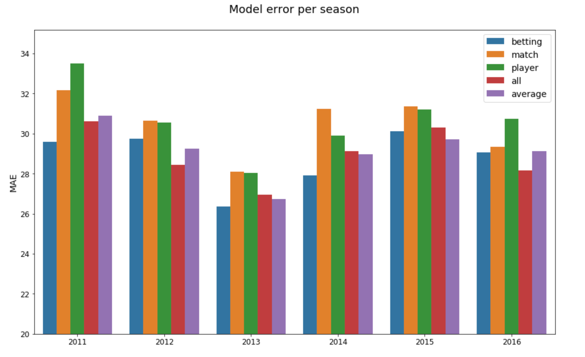
Well, that was underwhelming. The averaging ensemble managed to get the lowest mean absolute error for one season (2015), whereas the betting-data model had the lowest error for three seasons, and the all-data model won the two remaining seasons. One of the main advantages of ensemble models is that they have lower variance, so even though the averaging model only wins once, it comes in second three times and is never the worst model. However, if you take the mean error scores of the betting-data model and averaging model, the former comes out ahead with 28.80 to the latter’s 29.11. I tried adding the all-data model into the averaging ensemble, which did improve its error and accuracy slightly, but not enough to justify the addition of a whole bunch of parameters that would need tuning or the much longer training time, not to mention the headaches from being unable to fully utilise scikit-learn’s pipelines to organise my data and models. For the sake of thoroughness, I tested a simple stacked model (all of the non-average models feeding predictions into a basic XGBoost regression model), but, as expected, that performed even worse than the averaging model.
Feature engineering made easy
Though I must follow my boulder back down the hill, slapping the dust from my palms, rubbing the fatigue from my shoulders, I still manage to hum the happy tune that’s been stuck in my head for days. I recently read the book *Feature Engineering Made Easy* (FEME) by Sinan Ozdemir and Divya Susarla, and it gave me some ideas for my next attempt at the summit. I had already read a few books on machine learning, all of them doing a good job of teaching the fundamentals (the underlying math and algorithms, the basics of classification and regression, as well as useful tips and tricks for improving performance), but what I found particularly illuminating about FEME was in its change of emphasis: the authors largely (but not entirely) skipped over the fundamentals in order to focus on the trial-and-error workflow of developing machine learning models. Although I was already using cross-validation to compare the relative performance of different algorithms, model structures, and feature sets, in FEME, the authors add parameter tuning to their cross-validation process when comparing changes. This slows down the workflow of developing machine-learning models, but it also gets the results a little closer to the final performance, offering a more-accurate portrayal of each model’s error, accuracy, etc. once it has been tuned and is ready for production. When starting out, I would probably prefer the quicker feedback, but now that I’m working with ensemble models, with their myriad parameters, a little tuning can make a big difference, and the default values might not be giving me a good idea of how well these different models will actually perform.
Another bite at the apple
With this new strategy in mind, I went back to comparing different models, again using the basic all-data model as a benchmark, but with two important differences: using the joined data as a single input instead of juggling multiple data sources, and adding randomized search parameter tuning to the cross-validation. The simplified structure made it much easier to set up the averaging model and stacked model, such that I even added a basic bagging model (with XGBoost regressor as the estimator) to the mix. I chose randomized search over grid search, because, depending on how many iterations one uses, it’s much faster, and according to the scikit-learn documentation, under the right circumstances, it is almost as good as grid search for finding the best combination of parameter values. Doing k-fold cross-validation across the entire data set up to 2015 (as opposed to the yearly cross-validation of the previous trial), the performance of the averaging regressor, even with the sparse data, was now noticeably better than the all-data model, achieving an MAE of 26.53 while the latter got 26.88. Meanwhile, the bagging model scored 26.54 and the stacked model got 26.73. So, it looks like the averaging model and the bagging model have similar performance, but how close are they really, and are they really better than the much simpler all-data model?

Bringing statistics back
Another good recent read for me has been the paper “Model Evaluation, Model Selection, and Algorithm Selection in Machine Learning” by Sebastian Raschka. Unsurprisingly, since I’ve read his book *Python Machine Learning*, I was already familiar with most of the techniques and recommendations in the paper. His survey of statistical testing techniques, however, were new to me and of particular interest given my recent experiences with damn-near-impossible-to-parse performance differences among different algorithms. In this case, the question is one of the significance of differences in mean absolute error (MAE). How likely is a reduction of 0.25 in the MAE due to random chance? Does a difference of 0.01 MAE mean anything at all? Thankfully, I now know about the 5x2cv combined F test for measuring the statistical significance of differing performance scores for two models. What’s more, Raschka’s Python package mlxtend includes a function to get the F-value and p-value from this test, and it plays nice with the scikit-learn API. Running the test on ensemble models, using a respectably large data set, was kind of slow, but yielded interesting results. First, I compared the averaging and bagging models, getting a p-score of 0.5782, meaning any difference in their respective performances has a 57.8% chance of being due to randomness. I’m just using this score as an additional datum in determining which model I want to proceed with, so I wasn’t planning on holding myself to the usual 0.05 threshold, but having less than a 50% chance of being a real effect is a strong indication that I should use the simpler of the two, namely the bagging regressor which will require less tuning. With the same principle in mind, I used the F test to compare the bagging model to the all-data model, getting a p-score of 0.0007, which indicates that the bagging model’s better performance is probably worth the extra complication and slower training. As a side note, Raschka mentions the potential pitfalls of using pairwise tests like the 5x2cv combined F test and recommends using the Bonferroni correction. Again, I’m not being super scientific here, but just out of curiosity, if we apply the correction to the p-scores (i.e. dividing the target p-score by the number of times we performed the test), the difference between bagging and all-data is still well below the threshold for significance, 0.0007 being far less than 0.025.
The proof is in the (year-based cross-validation of) performance
Although, I’ve basically made up my mind to use a bagging regressor, for the sake of completeness, I scored the predictions for the bagging and averaging models for seasons 2011 to 2016 broken down by year.
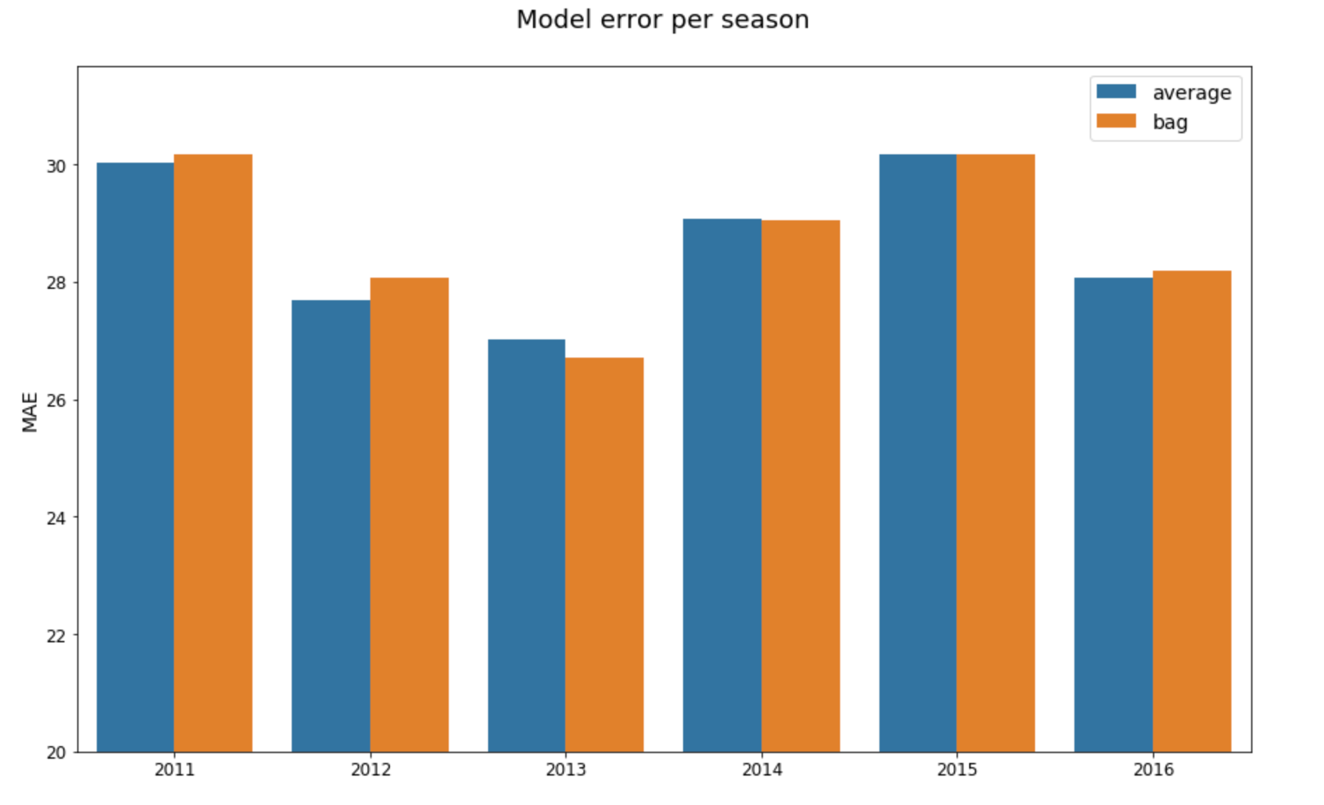
As expected, the models’ error scores are pretty close, with each winning three seasons. The bagging model performs a little better when looking at accuracy, winning four seasons, but the difference is small enough to be chalked up to chance. The overall averages across all of the measured seasons bear this out, with averaging getting a slightly lower error overall, and bagging getting a slightly higher accuracy.
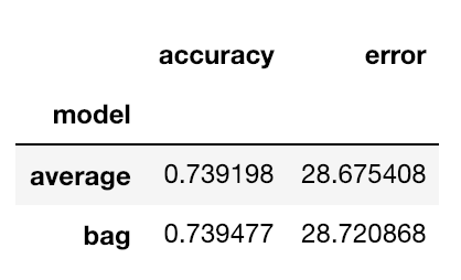
These figures provide the final evidence that there is no meaningful difference between the two models’ performances, so I’m better off using the simpler of the two, which, as stated earlier, is the bagging regressor.
For the umpteenth time: keep it simple, stupid
Well, my big idea came to naught, but I continue to learn the value of starting out simple and expanding from there rather than aiming for a big escherian target only to find out the folly of toying with non-euclidean nightmares that will overwhelm my feeble mind’s capacity for comprehension. One of these days, that lesson will stick. I’ve also learned the utility of applying statistical tests to machine-learning model scores to help with differentiating among them, which I will be sure to keep doing when basic cross-validation leaves the winner in doubt. Now that I have my ensemble model, I’m getting close to unleashing version 1.0 of tipresias on the world.